Seonghyun Park
Ph.D. student @ KAIST AI
hyun26@kaist.ac.kr
Bio
Hello! I'm a 2nd year Ph.D. student at Kim Jaechul Graduate School of AI at KAIST, advised by Sungsoo Ahn. My research interests are mainly on AI4Science, integrating machine learning to advance scientific discovery on small molecules and proteins! I'm interested in the following topics:- Small molecule interactions (drug, ligand)
- Protein dynamics, Collective Variables (CVs)
- Graph Neural Networks (GNNs), Over-squashing
Publications
Most recent publications on Google Scholar.
† indicates equal contribution, ‡ indicates co corresponding author.
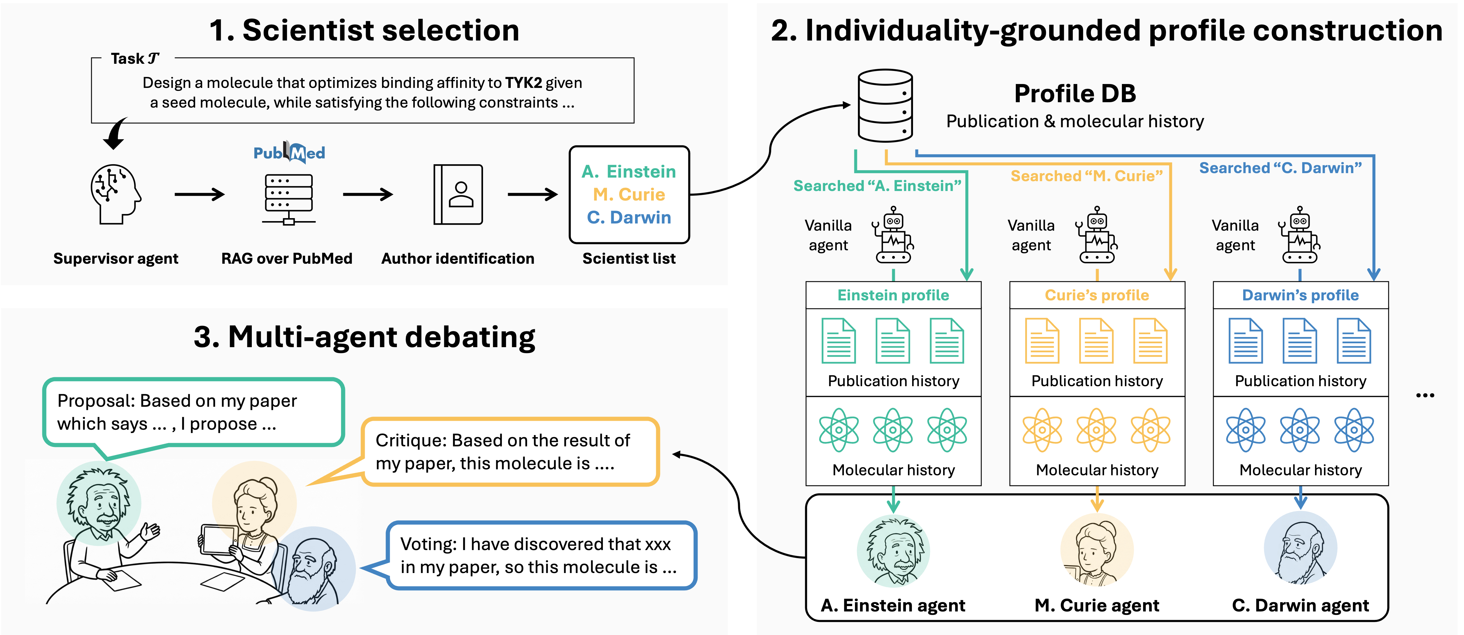
INDIBATOR: Diverse and Fact-Grounded Individuality for Multi-Agent Debate in Molecular Discovery
Yunhui Jang, Seonghyun Park, Jaehyung Kim, Sungsoo Ahn
Preprint, under review
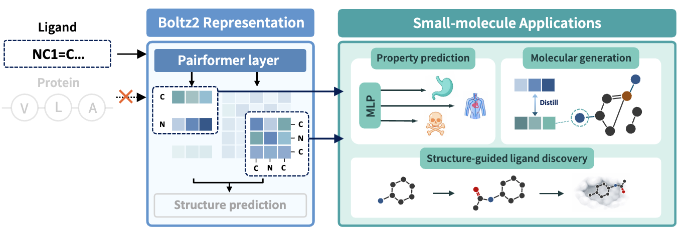
A Systematic Evaluation of Co-folding Model Representations for Small-Molecule Learning
Hyosoon Jang, Hyunjin Seo, Honghui Kim, Seonghyun Park, Taewon Kim, Yunhui Jang, Sungsoo Ahn
Preprint, under review
Dongyeop Woo, Marta Skreta, Seonghyun Park, Kirill Neklyudov, Sungsoo Ahn
ICML 2026
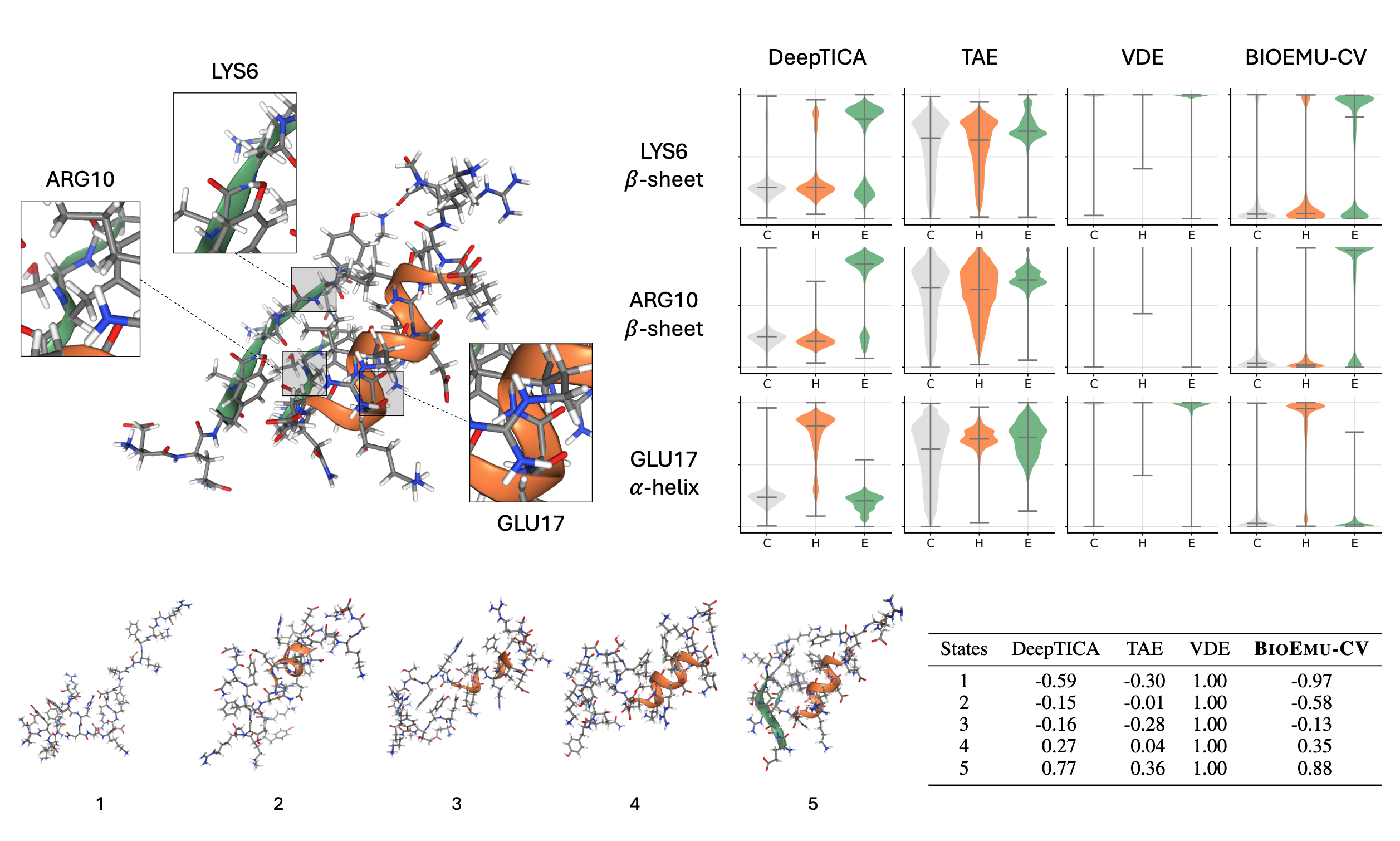
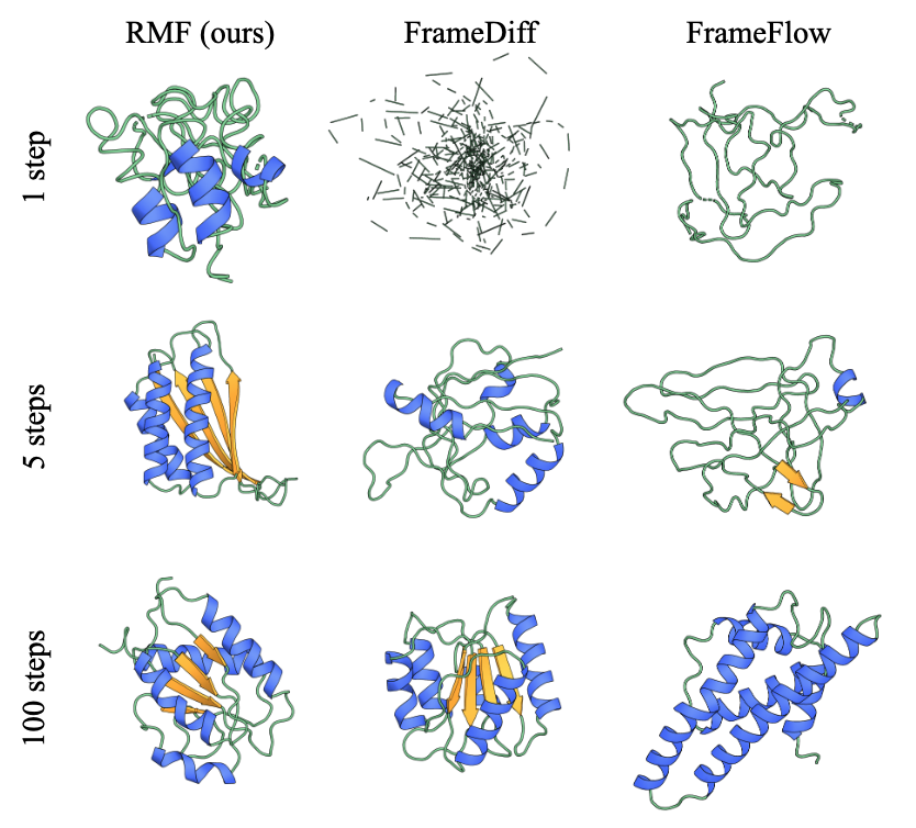
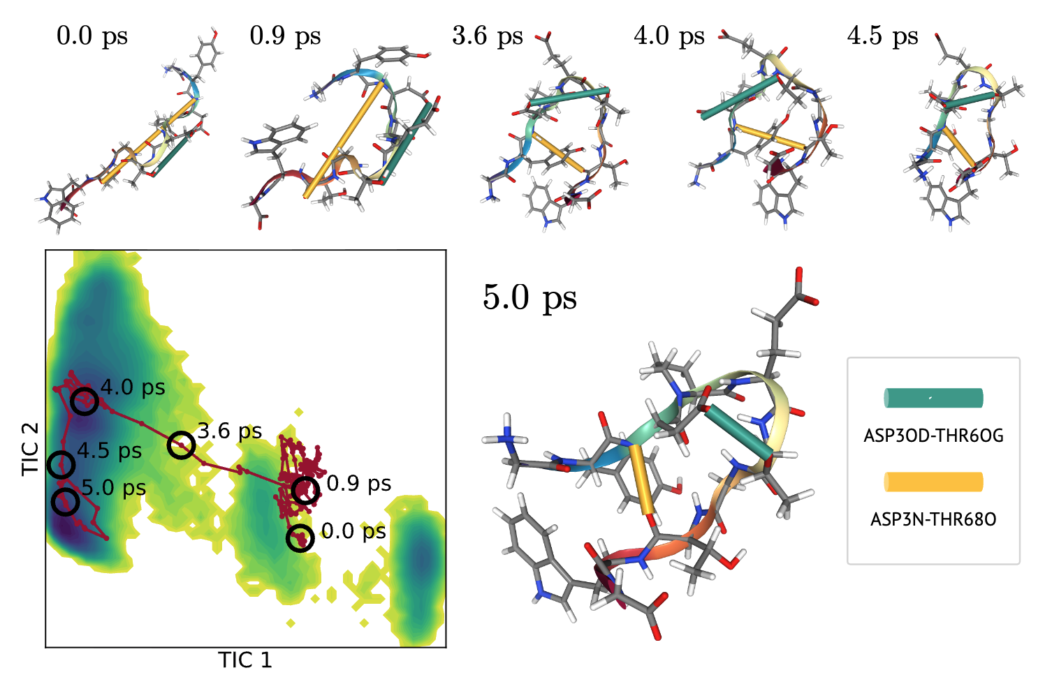
Learning Collective Variables from BioEmu with Time-lagged Generation
Seonghyun Park, Kiyoung Seong, Soojung Yang, Rafael Gómez-Bombarelli, Sungsoo Ahn
ICLR 2026
ICML 2025 Workshop, GenBio
Transition path sampling with improved off-policy training of diffusion path samplers
Kiyoung Seong, Seonghyun Park, Seonghwan Kim, Woo Youn Kim, Sungsoo Ahn
ICLR 2025
ICML 2024 Workshop, SPIGM
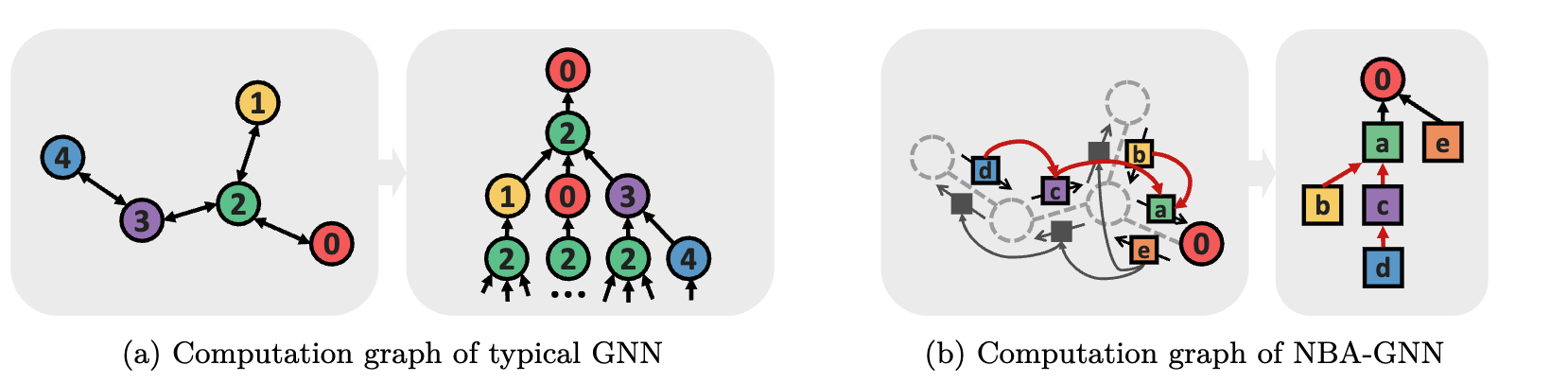
Non-backtracking Graph Neural Networks
Seonghyun Park†, Narae Ryu†, Gahee Kim, Dongyeop Woo, Se-Young Yun‡, Sungsoo Ahn‡
TMLR 2024
NeurIPS 2023 Workshop, New Frontiers in Graph Learning (GLFrontiers) (Oral)
INDIBATOR: Diverse and Fact-Grounded Individuality for Multi-Agent Debate in Molecular Discovery
Yunhui Jang, Seonghyun Park, Jaehyung Kim, Sungsoo Ahn
Preprint, under review
A Systematic Evaluation of Co-folding Model Representations for Small-Molecule Learning
Hyosoon Jang, Hyunjin Seo, Honghui Kim, Seonghyun Park, Taewon Kim, Yunhui Jang, Sungsoo Ahn
Preprint, under review
Dongyeop Woo, Marta Skreta, Seonghyun Park, Kirill Neklyudov, Sungsoo Ahn
ICML 2026
Learning Collective Variables from BioEmu with Time-lagged Generation
Seonghyun Park, Kiyoung Seong, Soojung Yang, Rafael Gómez-Bombarelli, Sungsoo Ahn
ICLR 2026
ICML 2025 Workshop, GenBio
Transition path sampling with improved off-policy training of diffusion path samplers
Kiyoung Seong, Seonghyun Park, Seonghwan Kim, Woo Youn Kim, Sungsoo Ahn
ICLR 2025
ICML 2024 Workshop, SPIGM
Non-backtracking Graph Neural Networks
Seonghyun Park†, Narae Ryu†, Gahee Kim, Dongyeop Woo, Se-Young Yun‡, Sungsoo Ahn‡
TMLR 2024
NeurIPS 2023 Workshop, New Frontiers in Graph Learning (GLFrontiers) (Oral)
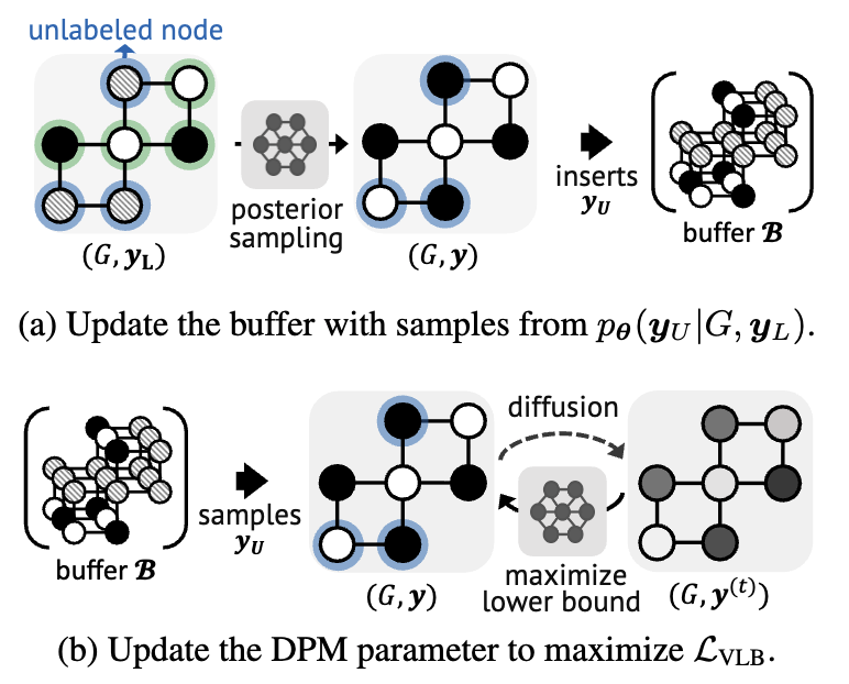
Diffusion Probabilistic Models for Structured Node Classification
Hyosoon Jang, Seonghyun Park, Sangwoo Mo, Sungsoo Ahn
NeurIPS 2023
ICML 2023 Workshop, Structured Probabilistic Inference & Generative Modeling
Side Projects
AMD
Automating Molecular Dynamics
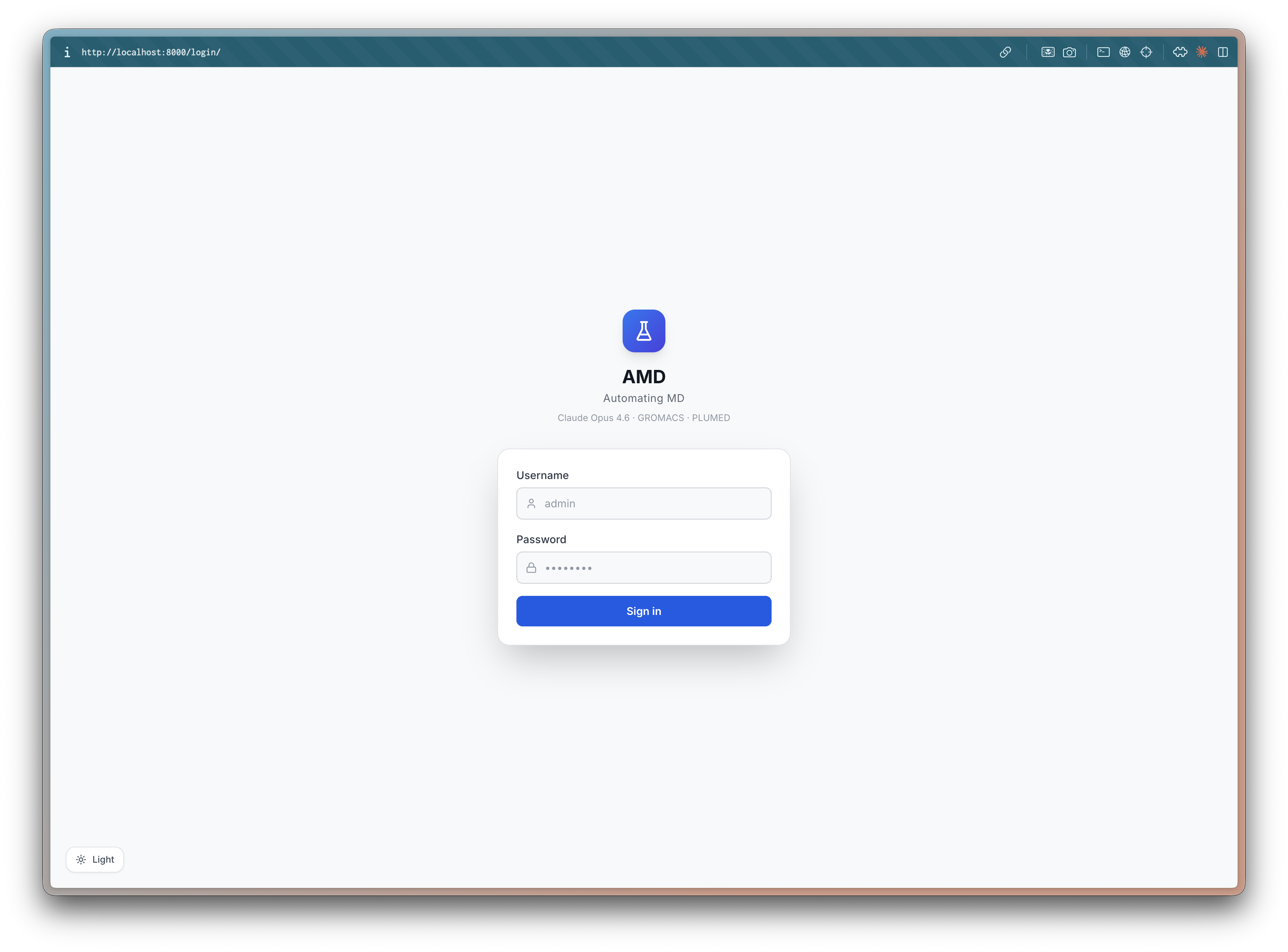
AMD is a localhost web application for running GROMACS + PLUMED molecular dynamics simulations through a browser GUI. Configure parameters, visualize molecules, launch simulations, and analyze results — all without touching the command line. Runs locally on your machine via Docker.
1. Log In
Open http://localhost:8000 and sign in. Each user gets their own sessions and settings stored in a local SQLite database.
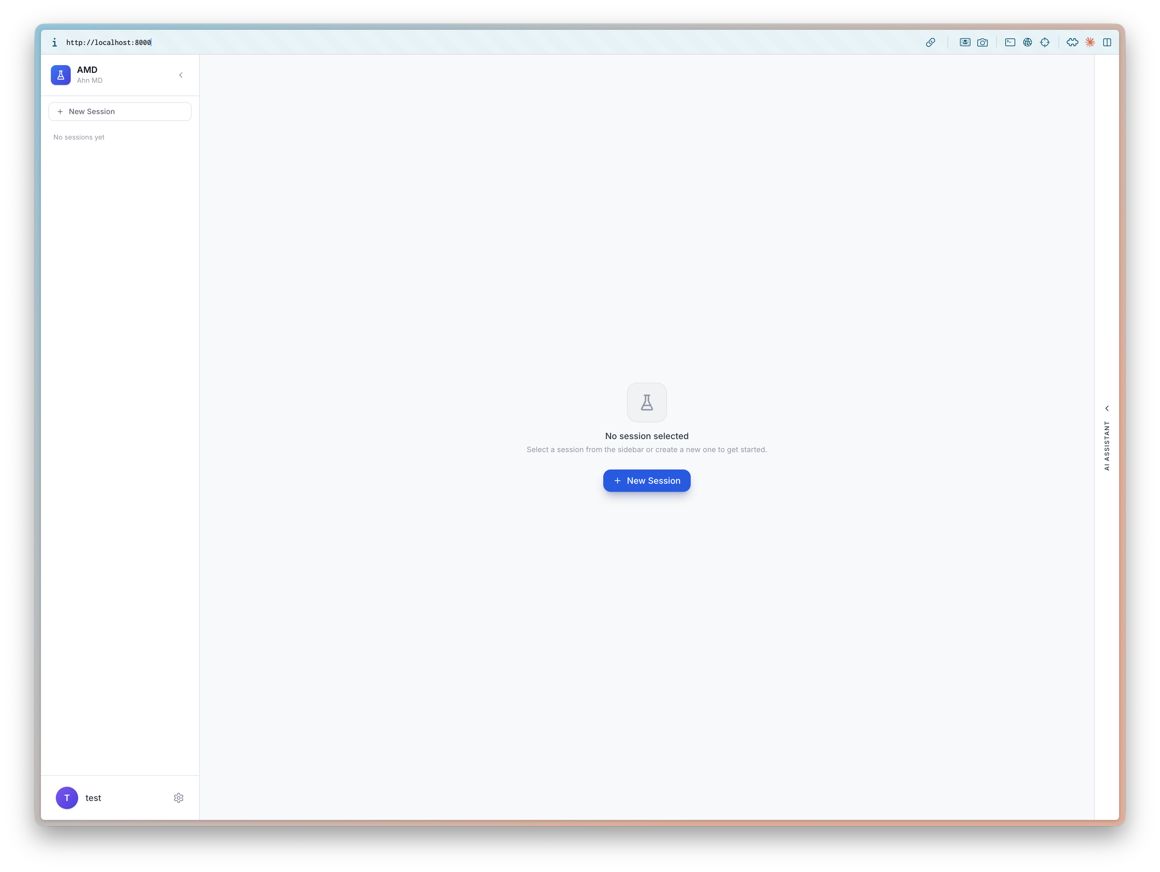
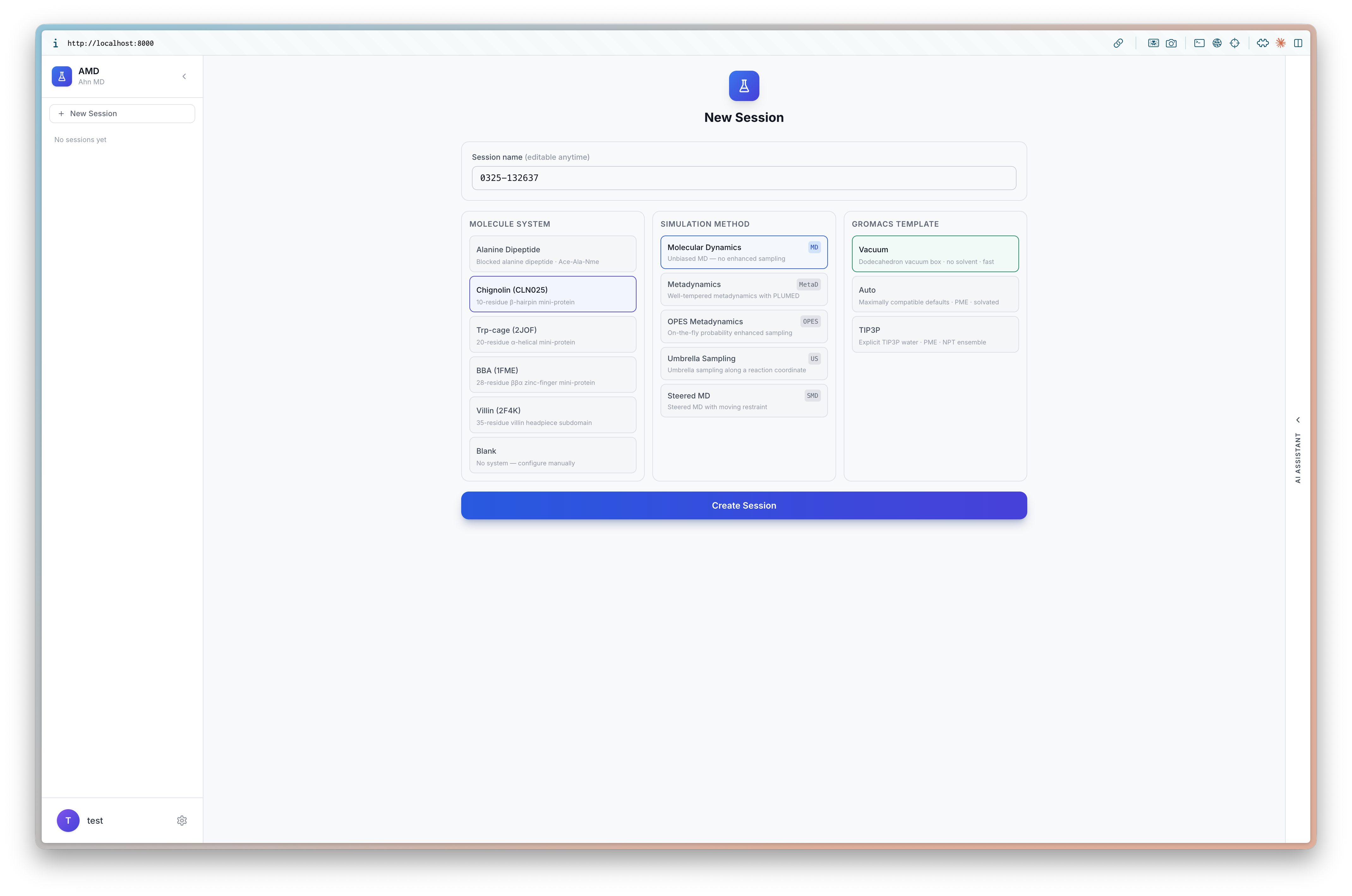
2. Create a New Session
The main dashboard shows a sidebar for managing sessions. Click + New Session to start.
The session creation screen lets you configure three things:
- Molecule System — Alanine Dipeptide, Chignolin (CLN025), Trp-cage, BBA, or Blank for custom uploads
- Simulation Method — Molecular Dynamics, Metadynamics, OPES, Umbrella Sampling, or Steered MD
- GROMACS Template — Default, Quick, Long, or Total presets that auto-fill parameters
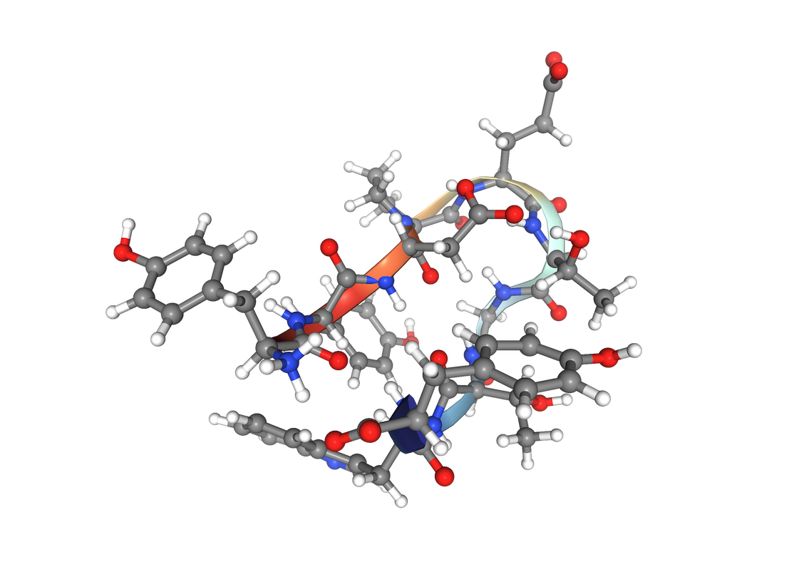
For this tutorial, select Chignolin (CLN025), Metadynamics, and the Default template.
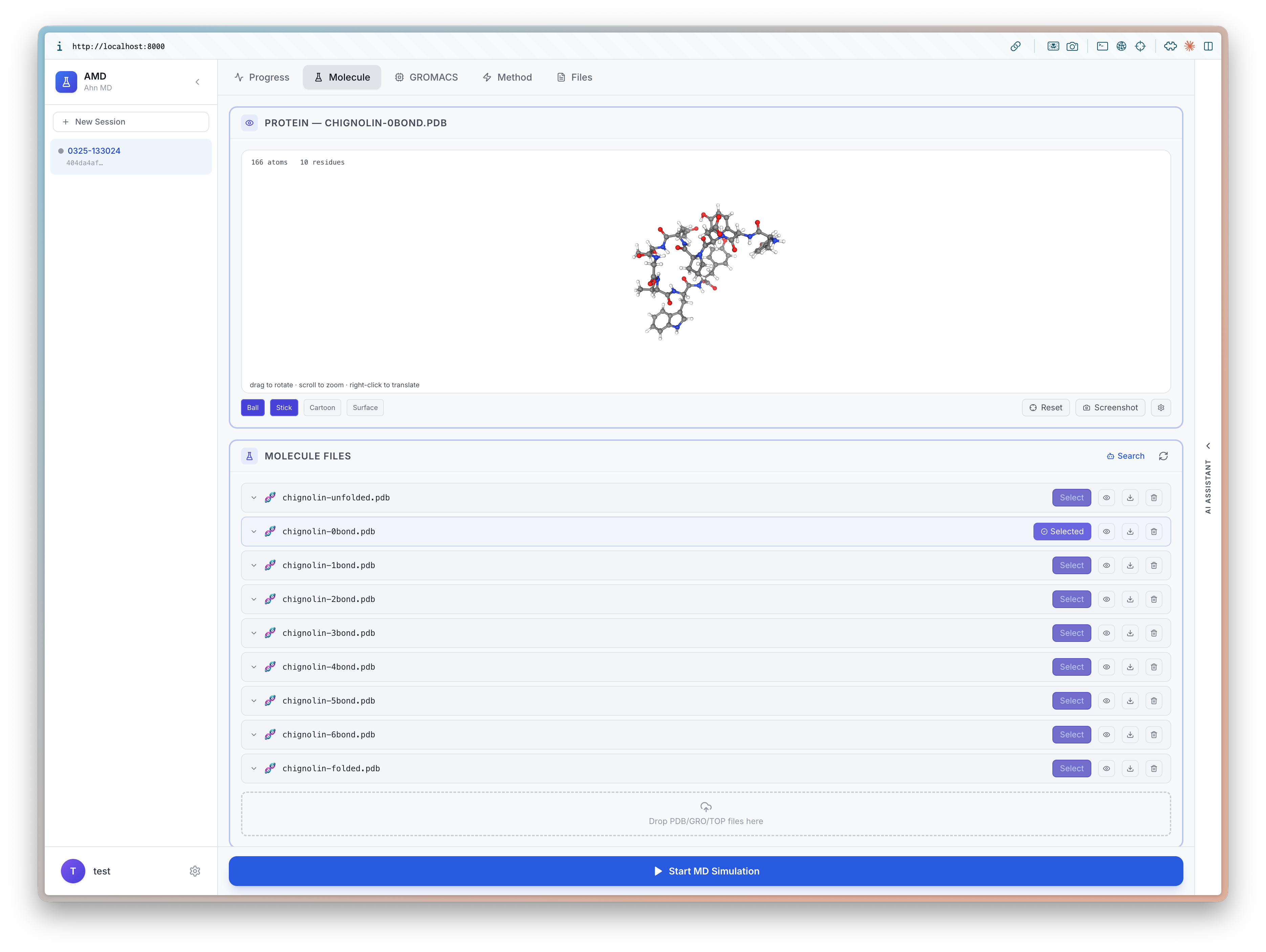
3. Load and Inspect the Molecule
The Molecule tab renders chignolin in an interactive NGL 3D viewer with Ball+Stick, Cartoon, and Surface representations.
Below, the Molecule Files panel lists all PDB files — original structure, processed conformations, and topology files. Upload additional files by dragging them in, or search RCSB directly.
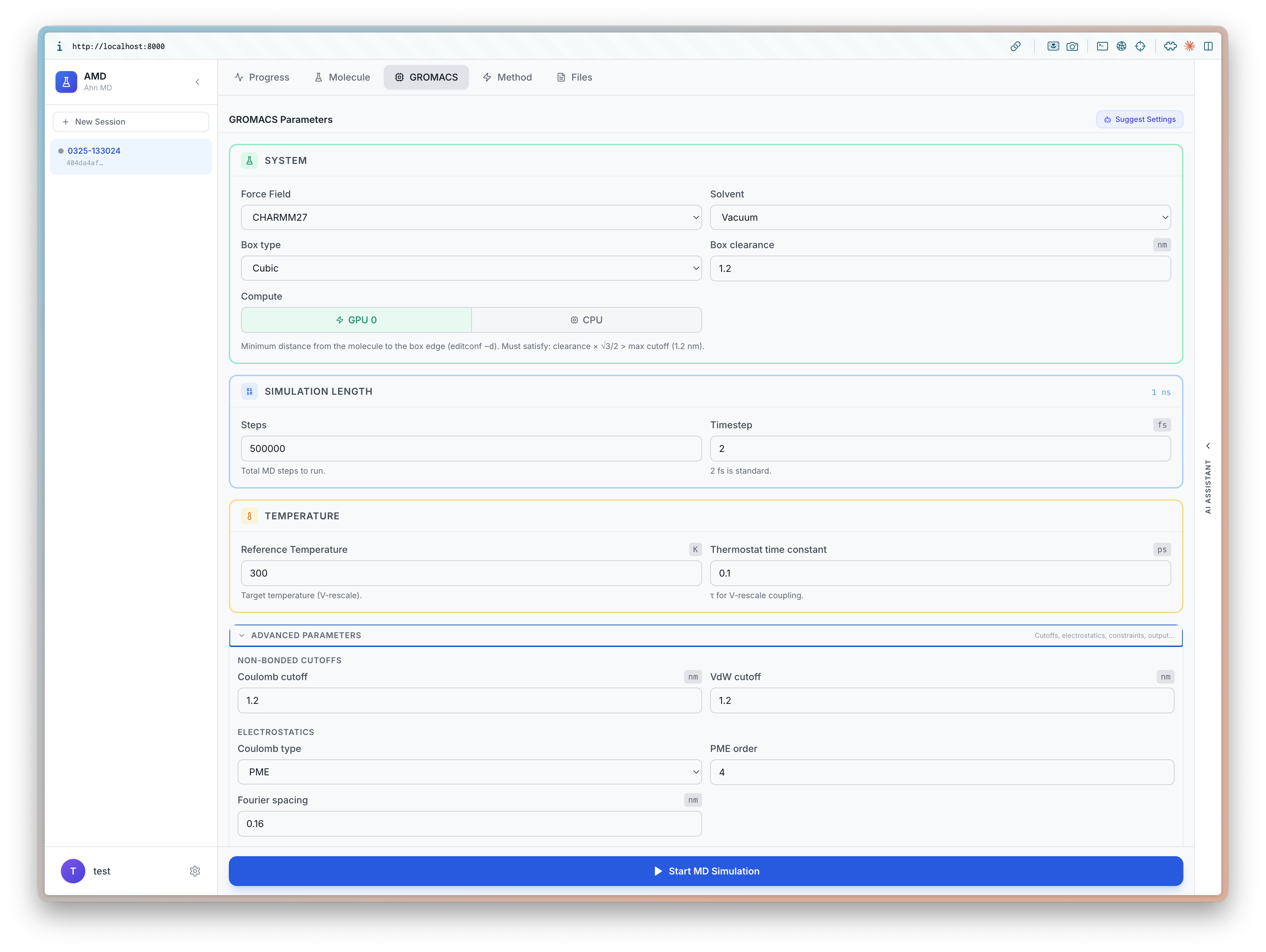
4. Configure GROMACS Parameters
The GROMACS tab provides full control over simulation parameters:
- System — force field (CHARMM27), solvent (Vacuum), box type (Cubic), box clearance, compute device (GPU/CPU)
- Simulation Length — number of steps (500,000) and timestep (2 fs)
- Temperature — reference temperature (300 K) and thermostat time constant (0.1 ps)
- Advanced Parameters — Coulomb/VdW cutoffs, electrostatics type (PME), PME order, Fourier spacing
Suggest Settings (TBA) — AI-powered parameter recommendations based on your molecule system and simulation method.
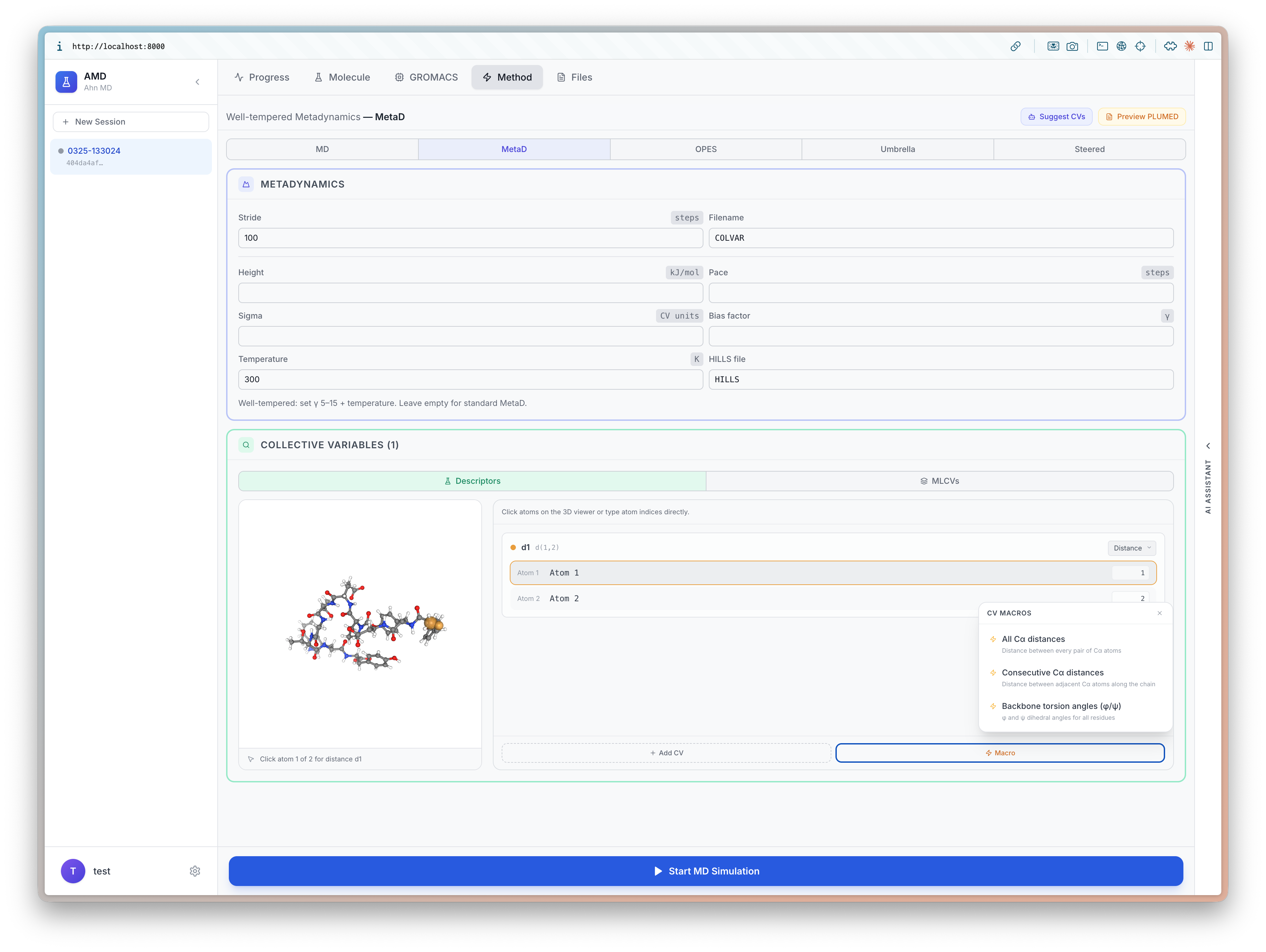
5. Set Up Metadynamics
The Method tab configures PLUMED enhanced sampling. Tabs at the top switch between MD, MetaD, OPES, Umbrella, and Steered.
For well-tempered metadynamics, set:
- Stride and Cutoff for hill deposition
- Height and Pace of the Gaussian hills
- Sigma and Bias factor for well-tempered behavior
- Temperature — must match the GROMACS thermostat
The Collective Variables section lets you define CVs interactively — click atoms on the 3D structure, or choose from presets: All CA distances, Consecutive CA distances, Backbone torsion angles (phi/psi), or custom selections.
Suggest CVs (TBA) — AI-assisted collective variable recommendations based on the molecule and sampling method.
Preview PLUMED — Preview of the PLUMED input file before launching.
6. Launch the Simulation
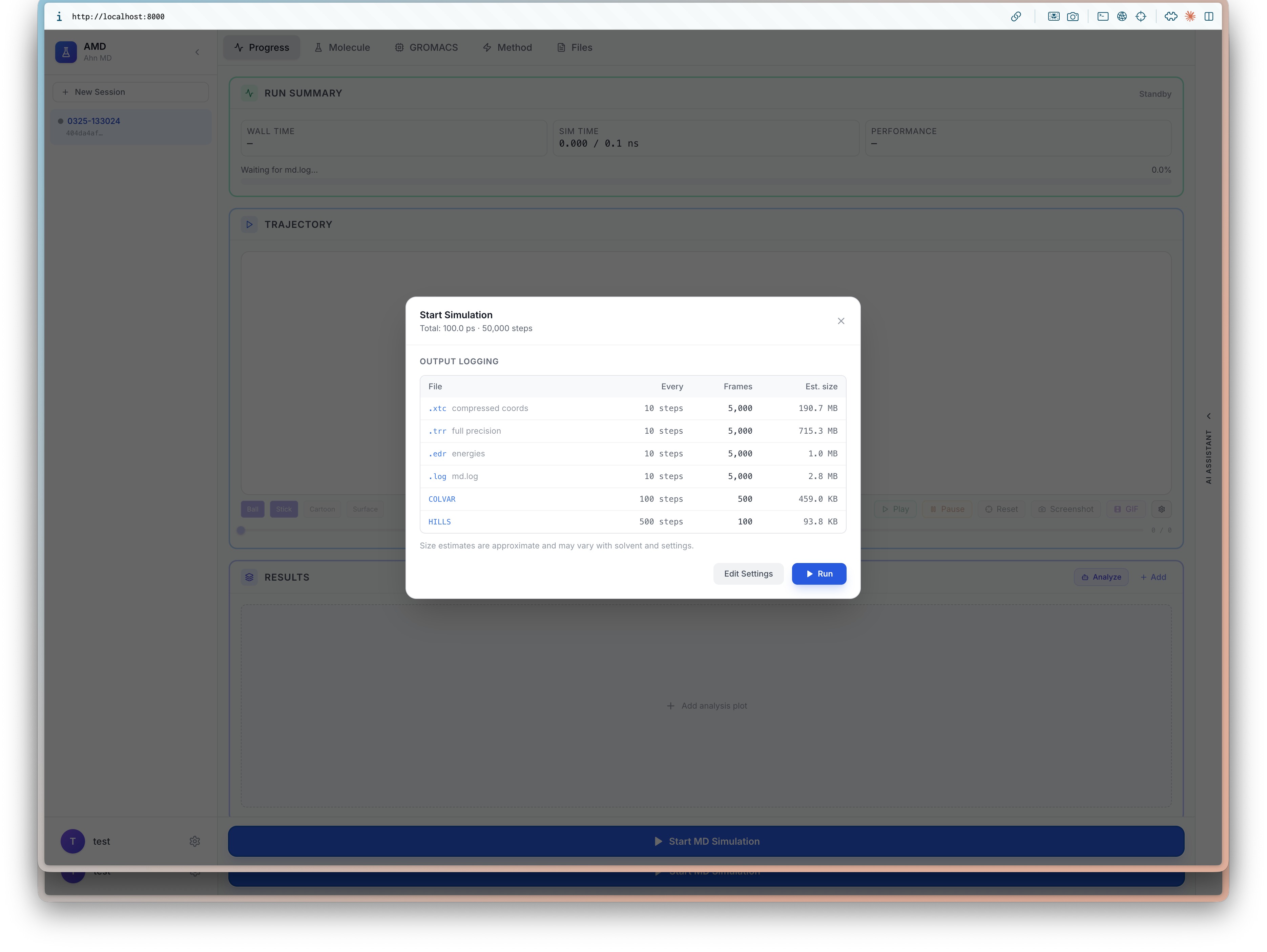
Click Start MD Simulation to see a summary dialog before running. It shows:
- Total simulation time and step count
- Output logging — each output file with its write frequency, number of frames, and estimated file size (e.g.,
xtccompressed trajectory at 10-step intervals,edrenergy file,logfile,HILLSandCOLVARfrom PLUMED)
Review the estimates, then click Run to launch. You can also go back to Edit Settings if anything needs adjustment.
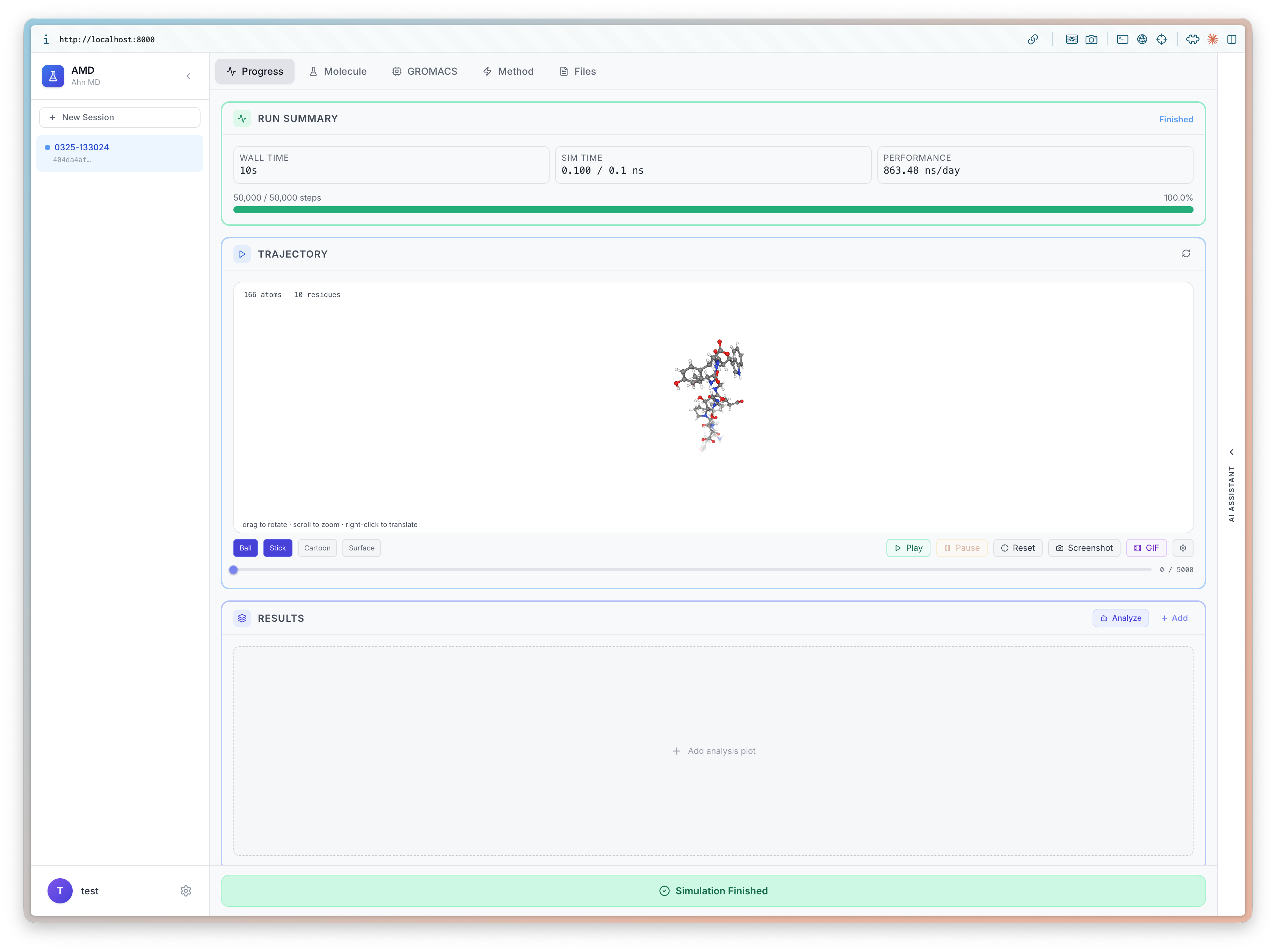
7. Track Progress
While running, the Progress tab updates in real time:
- Run Summary — wall time, ETA, and performance (ns/day)
- Progress bar — current step out of total with completion percentage
- Trajectory — live 3D viewer showing chignolin after simulation has finished, with play/pause, reset, screenshot, and fullscreen controls
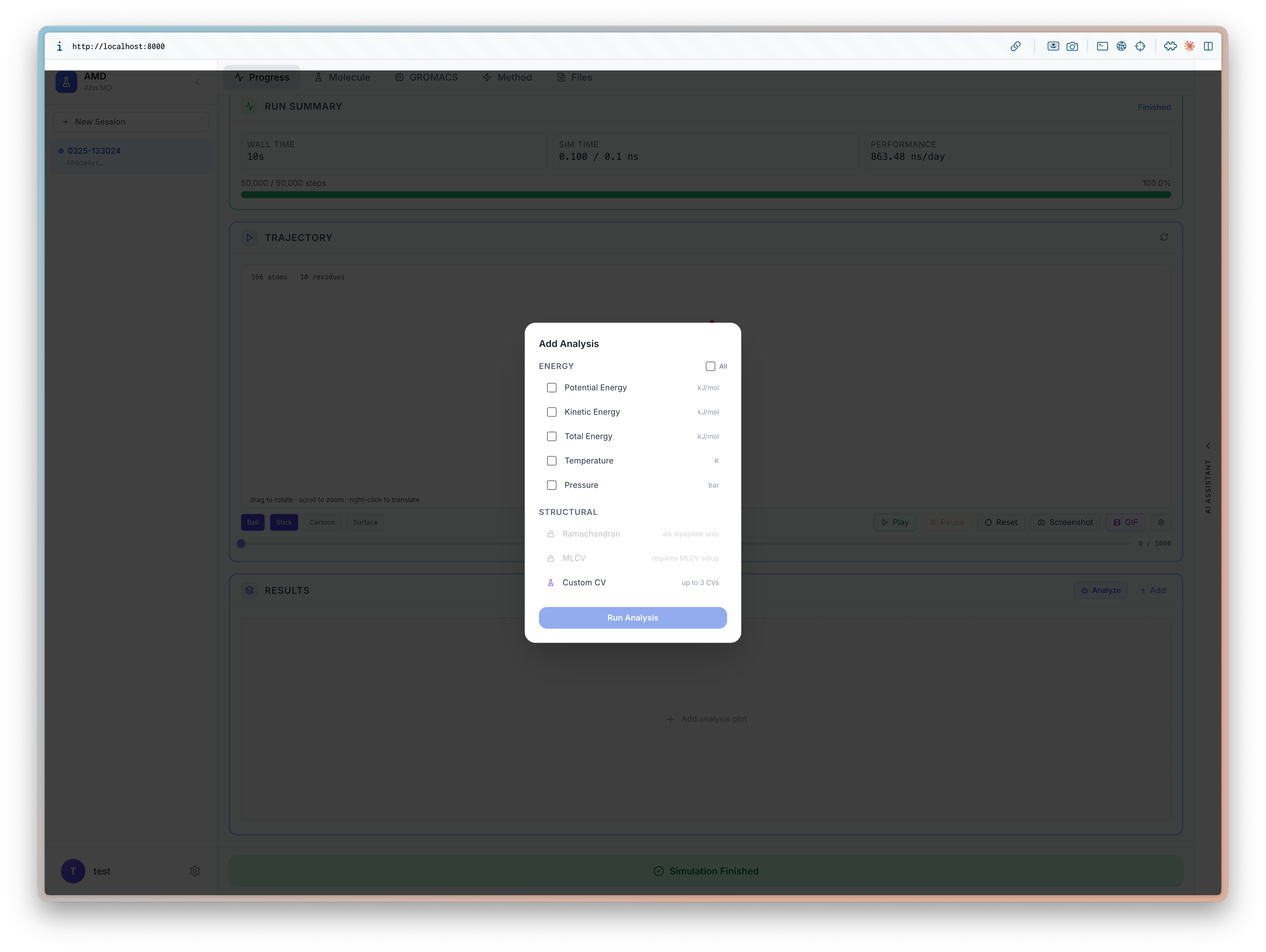
8. Analyze Results
Once the simulation finishes (green Simulation Finished banner), click + Add in the Results panel to select analyses such as potential energy, pressure, and Ramachandran plots.
Select the plots you want and click Run Analysis to generate them.
The Results panel then displays all analysis plots side by side — CV scatter plots, RMSD over time, pressure fluctuations, total energy, and more. Each plot is interactive and can be resized or rearranged.
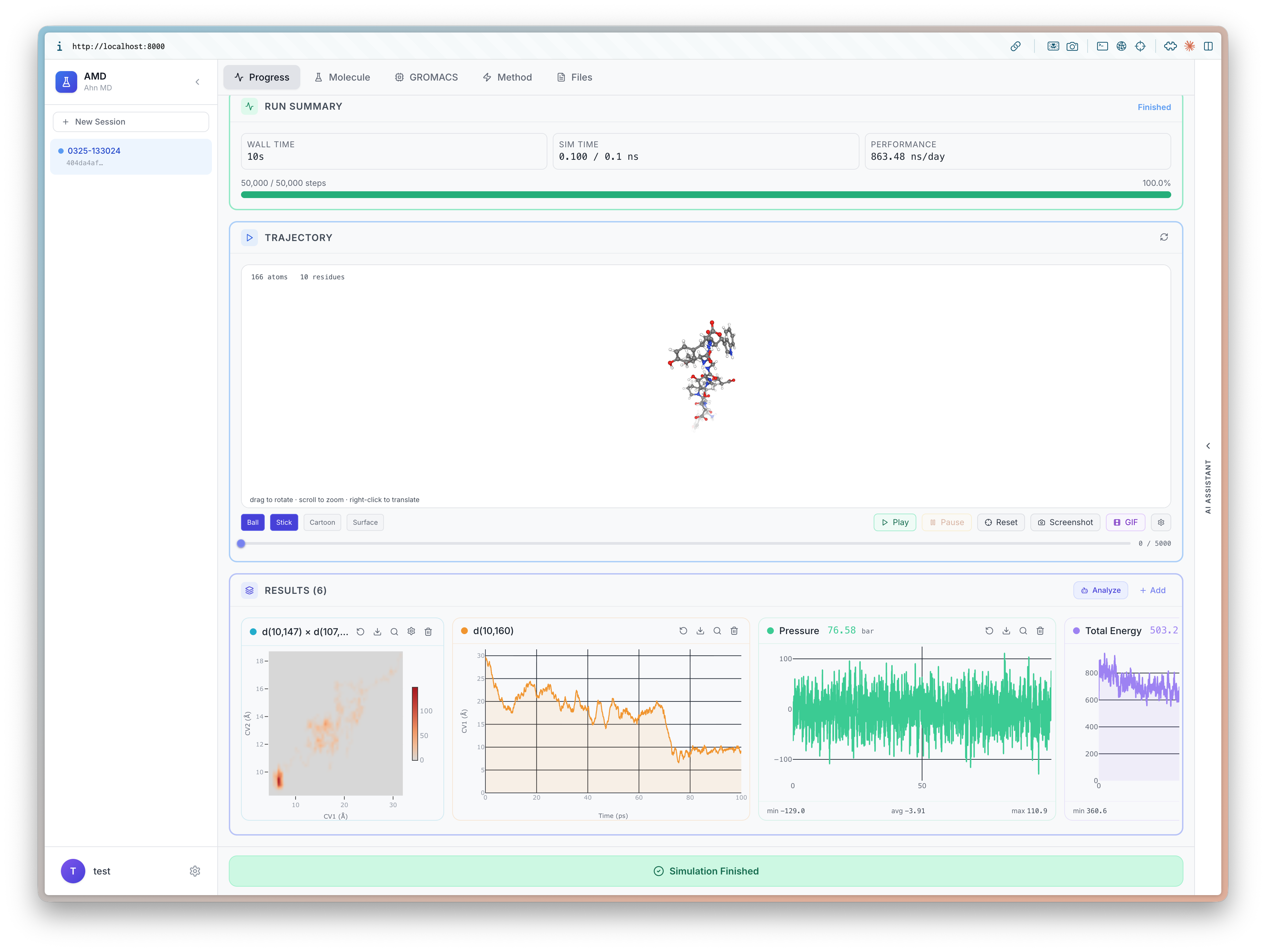
AI Analysis (TBA) — automated interpretation of simulation results, identifying metastable states and convergence.
Tech Stack: TypeScript · Python · Jupyter Notebook · Shell
License: MIT
Vitæ
Full Resume in PDF.
-
KAIST AI 2025 -Ph.D. Student
Structured and Probabilistic Machine Learning (SPML) Lab -
POSTECH 2023 - 2025Master's Degree
Machine Learning (ML) Lab -
INSA Lyon Spring 2022Exchange student
Bioinformatique -
Bagelcode Summer 2021Buisness Analyst, Intern
BA Team -
Sellerhub Summer 2020Product Manager, Intern
PM Team -
POSTECH 2019 - 2022Bachelor's Degree
Computer Science and Engineering
Hobbies 🎶📷
↑ Click this!